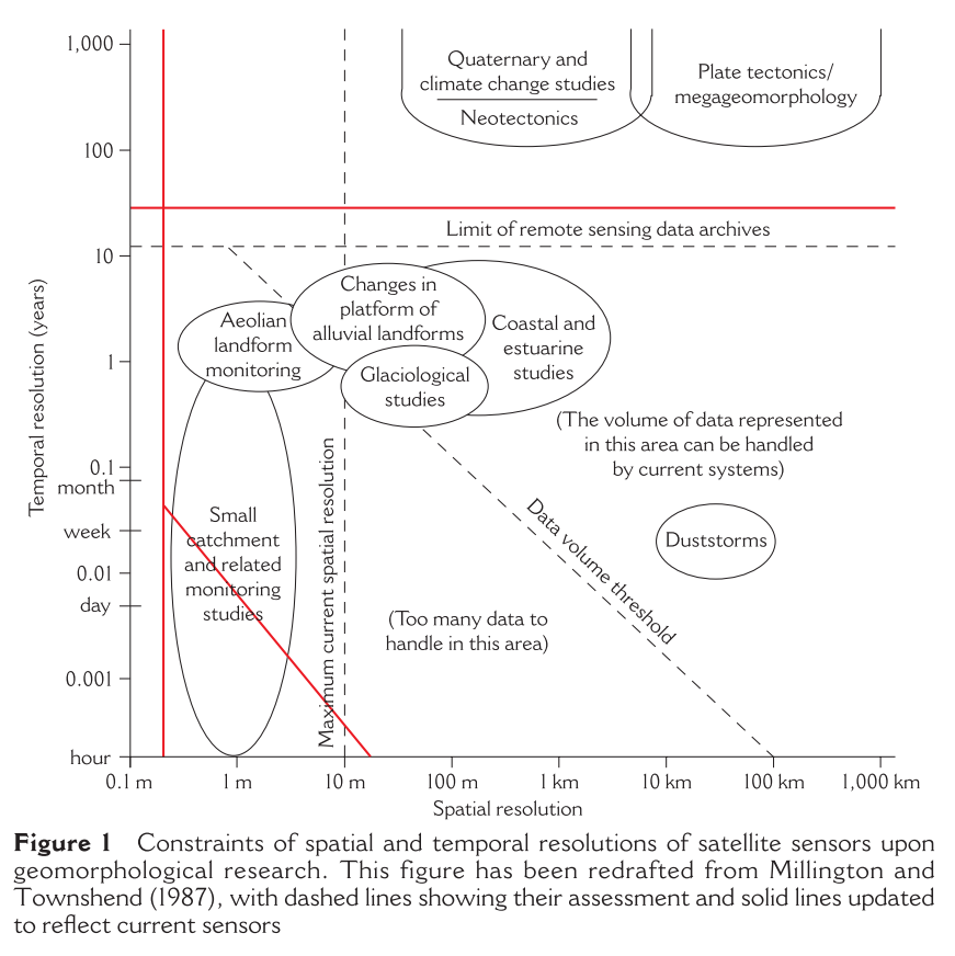
5.3 Geomorphology

5.3.1 Hess et al, 1990

“Radar detection of flooding beneath the forest canopy: A review” (Hess, Melack, and Simonett 1990)

Key significance: This reviews many of the earliest studies that employ SAR imagery for mapping of inundated versus non-inundated forest types.

Key notes:

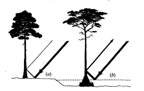
Of key importance for mapping of flooded vs. non-flooded forests is the fact that SAR imagery has a much more intense return off of water versus dry soil or trunks. Thus, the “double-bounce” effect off of a water surface is much stronger than that from soil & then tree.

An excellent schematic of this effect is shown below:

Accuracy of flood detection

Some have found an issue in that canopy that is too dense may attenuate the signal at too great of a degree, and thus the difference between the more intense return from flooded forests may not be apparent (L-band).

Additionally, presence of herbaceous vegetation (e.g., salt marshes) adjacent to flooded forests may erroneously appear as “flooded” forest using L-band. The bright return may be a result of the fleshy, vertically-oriented leaf stalks. These areas are still flooded, however, and thus it may still be effective for mapping of flooding extent, perhaps just not between flooded forest vs. flooded non-forest.

Magnitude of enhancement

Enhancement from flooded forest may range from approximately 2 - 10 dB.

Effect of radar parameters

Of primary importance are three considerations:

1. Incidence angle - angles at which imagery is collected vary greatly, and may be an important parameter for efficacy of detecting flooding
   • The most effective angle may depend on the ecosystem type. Flooded forests versus swamps may exhibit different dominant backscattering mechanisms.
2. Polarization - the polarization of the radar may effect the efficacy of the return in identifying inundated landscapes
   • Majority of studies have used HH polarization (Seasat, SIR-A, SIR-B)
   • Qualitative assessments are consistent in findings that like-polarized scenes (HH or VV) are more effective at identifying flooded forests via L-band
3. Frequency - use of P-, L-, or X-band may have different dominant backscattering mechanisms, and thus may influence detection of inundation.
   • L-band commonly used due to ability to penetrate dense canopies, however may have some limitations
   • P-band may be promising for mapping of inundated forests in forests that are very tall or with very dense canopies

Applications in flooded forest research

Critical to examine the temporal and spatial variability of water cover. An important component is availability of ground data on extent and time of flooding at the time of imaging, particularly tricky for tidally inundated forests.

Additionally, for forests with aboveground root structures (i.e., mangroves), scattering of the signal by aboveground roots may reduce the signal and reduce ability to identify inundated forests.

5.3.2 Walsh, 1998

“An overview of scale, pattern, process and relationships in geomorphology: A remote sensing and GIS perspective” (Walsh, Butler, and Malanson 1998)

Key contribution: This study exemplifies the “scale, pattern and process paradigm” for exploration of geomorphological relationships in two study systems: alpine and fluvial environments. The authors note the value of remote sensing and GIS, as well as their integration, for examining processes that may occur over different scales.

The authors note the basic intent of the study is to examine use of space-time scales for organizing and examining geomorphic and biogeographic processes via a RS-GIS system framework.

Key notes:

The study is motivated by early theoretical work in landscape ecology, which functions largely under the premise that ecological patterns and processes are largely dictated by the spatial arrangement and patterning of a landscape.

The authors note several key values of GIS work for landscape processes, in particular:

1. Examination of spatial vs. non-spatial relationships via explicit tools (overlays, etc.)
2. Represent an array of landscape perspectives through integrating geographically registered spatial coverages
3. Efficient display of information
4. Examine co-occurrence of spatial and non-spatial data
5. Display singular thematic or composite coverages
6. Can model location and response of phenomena

Critical consideration is the scale at which ecological processes happen, and the scale of the dataset (e.g., 30 x 30m pixels) that one is working with.

The paper provides a review of remote sensing and GIS, which I have largely omitted here except for a few key points.

GIS can be used to produce spatial metrics (quantification of the composition and spatial pattern of landscape units), which may help assess degree of spatial organization within a landscape. As the authors refer to it, these are largely the precursor to what is now termed object based image analysis.

Landscape level pattern indices may include: dominance, contagion, fractal dimension, or lacunarity indices.

Lacunarity incorporates overall fraction of map covered by a phenomenon, degree of contagion, presence of self-similarity, scale of randomness and presence of hierarchical structure.

In essence, lacunarity describes the degree of similarity of regions within a geographic area at a predefined scale.

Spatial metrics at landscape level can be generally understood to provide information on landscape heterogeneity indices due to measurements of overall landscape structure within defined area.

GIS can also be useful for assessing scale dependencies. Semivariance and fractal dimensions are used to assess nature and degree of spatial autocorrelation within landscape elements over different spatial scales.

Examples of overall scale dependence that may influence a study are:

1. The precision with which scales and the region of interest are defined
2. Nature of the variables that are examined (local scale may be physical variables, regional may be climate or land use)
3. Degree of scaling (either up or down) that is attempted

Explicit recognition of the importance of scale has led to the use of hierarchy theory within landscape ecology studies (may want to read up more on this).

Fluvial case study

The authors describe the different scales of environmental processes that shape the meandering and development of alluvial systems. They note the importance of both spatial and temporal scales.

Fine spatial scales may be seen in channeling or sedimentation along particular points within a river, and are likely due to interactions of flow and sediment properties at fine scales.

At coarse spatial scales, development of abandoned channels are controlled by water flow across floodplains and proximity of site to the channel.

Additionally, for temporal scales, sharp pulses in water flow or longer term gradual shifts may have different effects on an alluvial system.

5.3.3 Imhoff, 1990

“The derivation of a sub-canopy digital terrain model of a flooded forest using synthetic aperture radar” (Imhoff and Gesch 1990)

Key significance: This is one of the earliest uses of SAR imagery to map digital terrain models and understand tidal inundation in a mangrove forest. The study couples both SAR imagery as well as field measurements of tidal inundation in a novel manner, and provides discussion of syncing the timing of imagery acquisition with hydrological records.

Key notes:

The study employed data from both the SIR-B mission as well as tide surface information to create a digital terrain model in southern Bangladesh.

They note the importance of hydrology and geomorphology on mangrove health, citing Lugo and Snedaker’s discussion in which they note that “tidal dynamics” and “water chemistry” are the two most important factors on mangrove health.

The radar data used for the study consisted of three HH polarized L-band radar images, acquired at 26, 46 and 58 degree angles of incidence.

The field data comprised of tide gauge data from five stations throughout the region slightly larger than the survey area, a 1,200 m topographic survey transect, and test plots in the forest that were visited during the radar data acquisition period.

DN counterparts to mean backscatter coefficients were used to select break points for classifying flooded versus non-flooded forests.

Results

All three datasets were coregistered, and field data were used to train a model on flooded vs. non-flooded forest areas.

A spatial filter was applied using a 5 by 5 and then 11 by 11 median filter to remove speckling. The processed image allowed for better discriminating between classes at a spatial frequency appropriate to the formation.

The 58 and 46 deg images were combined to produce an inundation map (the 26 deg data had issues during time of collection, but was used for validation of land edge boundaries), and subsequently into a topographic map.

In doing so they produced numbers along the inundation boundaries, which took on values of elevation level relative to mean sea level. The values of the pixels were used as points and an interpolation procedure was used to produce a continuous DTM.

The authors then discuss various sources of error, which include resolution issues, measurement error, as well as imprecise measures of “flooded” vs “non-flooded” forest recognition by the L-band SAR imagery.

5.3.4 Souza-Filho & Paradella, 2002

“Recognition of the main geobotanical features along the Bragana mangrove coast (Brazilian Amazon Region) from Landsat TM and RADARSAT-1 data” (Souza-Filho and Paradella 2002)

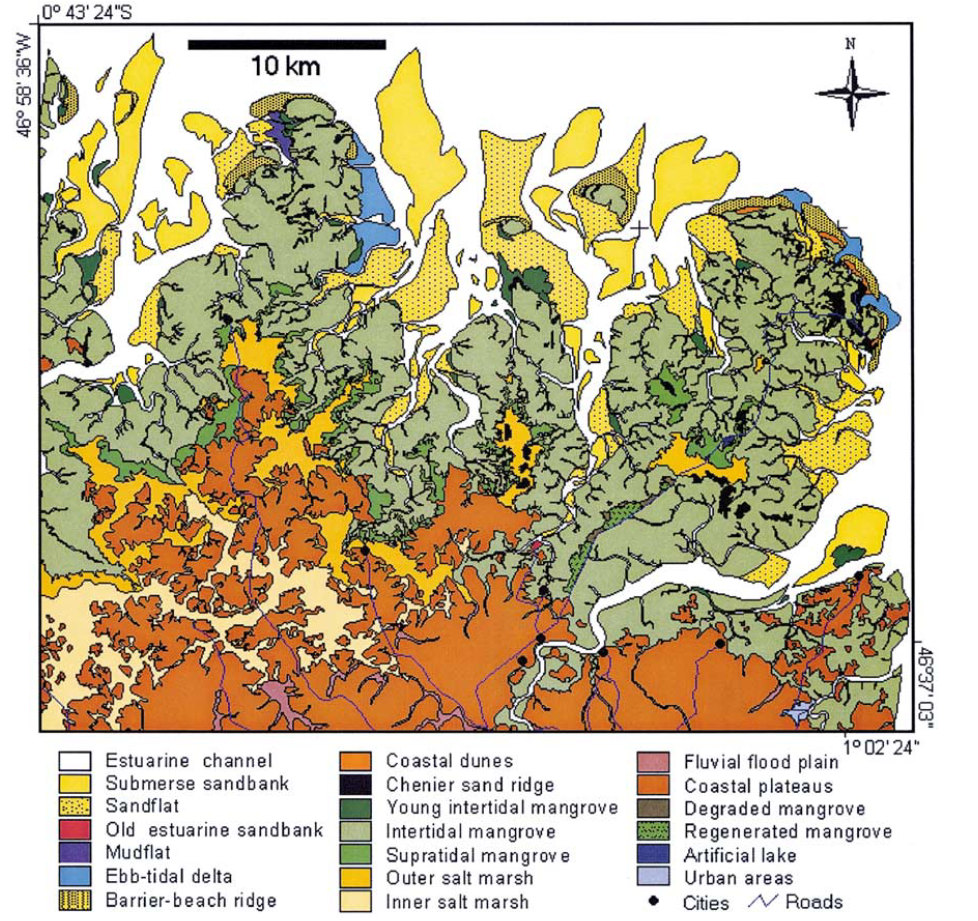
Key contribution: This study exemplifies integration of Landsat and SAR data for mapping of different ecosystem types and successional classes along the Bragana coastline at a landscape scale. Incorporation of landsat and SAR data enables mapping of not only different ecosystem types, but also successional classes (e.g., young vs. mature intertidal mangroves, degraded and renegerated mangroves, etc.).

Key notes:

The authors process Landsat TM and RADARSAT-1 SAR data, and build a composite product using an “Intensity, Hue and Saturation” transform. The transform uses a RGB/IHS transform that incorporates channels formed from PCA of Landsat bands 1, 3 & 3; bands 5 & 7; band 4; as well as an intensity band from the RADARSAT-1 data (described in Harris et al., 1994, Paradella et al, 1998, Pohl, 1998).

The resulting map incorporates the spectral data as well as the intensity data corresponding to SAR topography, with an array of colors and values across the landscape. Using field data and prior knowledge, the authors then visually interpret the map into a variety of different land features.

Key criticism - they do not provide a full accuracy assessment and thus it is unclear how accurate their results are. The map provides much more information (colors) than is interpreted, and thus it is unclear how legible the map necessarily is (classifications may be too fine scale).

They produce a map with 19 classes of the landscape, but it is unclear how they arrive at this point. Assuming that they used the integrated product and supervised classification.

Nevertheless, if we take the procedure for granted, they are able to distinguish between a variety of geobotanical features, including: channels, open water, mudflats, coastal dunes, young intertidal mangroves, intertidal mangroves, supratidal mangroves, degraded mangroves, outer salt marshes, and urban areas.

The final map classification as they provide it is shown below:

Conclusion

The methods are a little black-boxey and may require digging into the associated PhD thesis (in Portuguese), but the map is an interesting approach to pulling information from both spectral (Landsat TM) as well as radar-based (RADARSAT-1) information.

5.3.5 Souza-Filho, 2003

“Use of synthetic aperture radar for recognition of coastal geomorphological features, land-use assessment and shoreline changes in Bragana coast, Para, Northern Brazil” (Souza-Filho and Paradella 2003)

Key contribution: This study is a sister study to that of (Souza-Filho and Paradella 2002), and examines mapping of geomorphology as well as changes in coastal extents over time. The study uses SAR data acquired from over a 30 year period to investigate areas of coastal progradation versus erosion.

Key notes:

The difference in SAR return from land versus water is largely a function of contrast of dielectric properties as well as surface roughness, and allows for striking interface along coastal landscapes.

The two SAR imagery datasets used were airborne X-HH band data from 1972, and orbital (satellite-based) C-HH band data from 1998. Both images were acquired at high tide conditions.

Imagery were ortho-rectified based on ground points that were obtained during a field campaign.

The SAR imagery from 1972 was used to distinguish between terrain and open water, converted to a vector dataset, and overlaid on the 1998 imagery to examine changes in shoreline over time.

The authors provide a nice overview of the steps that must be taken for use of SAR data (i.e., processing):

1. Input data
   • Reading of image orbit data and 16 bit RADARSAT data
2. Preprocessing phase
   • Radiometric correction - scaling of 16 bits to 8 bits, ground control point selection
   • Geometric correction - math model for geometric correction, geometric ortho-correction + speckle reduction
3. Enhancement
   • Linear stretch
4. Assessment of SAR product
   • Radargeologic interpretation

Results - Mapping of land cover classes

The authors used visual interpretation to identify six prominent geomorphological coastal features. Intertidal vs. supratidal mangroves can be determined given different microwave responses to vegetation. Supratidal mangroves are shorter and more open, and thus result in a reduced double-bounce effect relative to intertidal mangroves.

They used aerial imagery in conjunction with the SAR data to help validate some of their land classifications.

Results - Mapping of shoreline change

Other studies have noted that mapping shoreline change during Spring High Tide Level is most appropriate, thus both images were acquired at same high tide condition.

The authors conclude that the shorelines has been subject to severe erosion, but I’m also not sure how they distinguish between this and sea level rise during the time period. They identify both areas of erosion as well as deposition, but with a net effect of erosion in the study region.

They note that deposition of sand has killed mangrove vegetation, and thus the mangrove terrace has largely been eroded.

They also note that in other areas, sediment supply and protection from wave attacks has allowed for accretion of sandbanks, muddy deposition and establishment of mangroves.

The full map or erosion and accretion in the area is shown below:

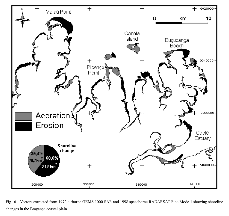
The authors use the maps of erosion and accretion coupled with ecosystems to understand processes that may be occuring within the landscape. The authors also note, however, that much of the findings are speculations given the absence of wind, wave, and tidal currents data within the region.

Time series analysis of SAR data thus may be informative in investigating long-term trends along coastlines, particular for identifying regions of erosion or deposition.

5.3.6 Knight, 2009

“Exploring LiDAR data for mapping the micro-topography and tidal hydro-dynamics of mangrove systems: An example from southeast Queensland, Australia” (Knight et al. 2009)

Key contribution: This is one of the very few studies that employs airborne LiDAR to derive a high resolution digital elevation model and examine inundation and hydrology characteristics within a mangrove forest.

Key notes:

The study was motivated by the need to map habitats for a disease vector mosquito.

The digital terrain model that they obtained had a vertical accuracy of 0.5 m, and was validated by using hydrological modeling and field data of tidal gauges over ten days.

The accuracy of the DTM and that of field data indicating habitats for mosquitos were found to validate one another.

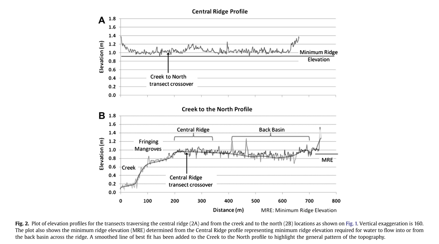
Of key geomorphological importance is the fact that they were able to identify a ridge that ran through the majority of the site as well as back basins and fringing mangroves. The back basin was blocked from tidal waters during all times except for the highest tides. Such understandings may be important for understanding the spatial ecology of a site.

The authors also note the importance of the LiDAR derived DTM for understanding effects of SLR on the mangrove forest.

Study design

LiDAR was flown over the area, producing a shapefile with 3 million points. The points were classified as ground versus non-ground by removal of points not contributing to ground terrain points by +/- 0.1 m. The ground point data was validated against GPS base-station data. 150 points were used to assess vertical accuracy across the entire area.

The tidal inundation data was collected from 10 points in the field, recording water depth, pressure and temperature every 5 minutes continuously for 10 days. Locations of the tidal gauges were informed by the DEM, selecting for areas near to tidal sources, in depressions or on hummocks. The tidal depths were used to validate inundation patterns expected given the LiDAR DTM.

Tidal inundation was modeled in ArcMap by “flooding” of the landscape in 0.05 m increments, with flooding constrained to adjacent to water bodies (i.e., the back basin was not flooded until the berm was breached).

Results

The use of the DTM was able to identify the presence of a berm as well as back basin. The below figure displays the findings. The top figure displays the elevation along a transect that was conducted along the center of the berm. A minimum elevation can be seen that must be breached for flooding of the back basin.

The total DTM for the site can be seen below:

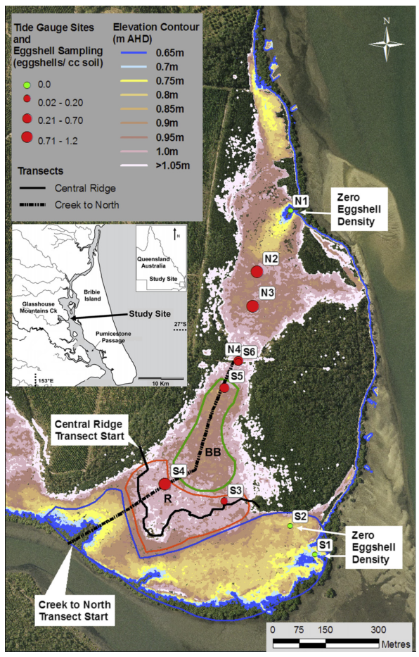
The authors conclude that use of LiDAR data for derivation of the DTM was successful, and that the approach that they took may work well for modeling of shifts in hydrology that may occur with sea level rise.

5.3.7 Smith, 2009

“Applications of remote sensing in geomorphology” (Smith and Pain 2009)

Key contribution: A review of the use of remote sensing for geomorphology, without a particular focus on mangroves. The article reviews the current platforms and data types, and maps them to their relevant uses within geomorphology.

Of particular note:

Remote sensing particularly well placed to aid studies of geomorphology in:

1. location and distribution of landforms
2. land surface elevation
3. land surface composition
4. subsurface characterization

The authors remark consistently on the added value of digital elevation models (both as products, as well as automatic classification by sensors) for geomorphology.

Among most important techniques for postprocessing of LiDAR point clouds for geomorphologists is removing “surface clutter” to extract actual ground surface.

Note:

• Look further into mangrove sites on OpenTopography

Further reading:

1. Clark, 1999 - Spectroscopy of rocks and minerals, and principles of spectroscopy
2. Sithole and Vosselman, 2004 - Experimental comparison of filter algorithms for bare-Earth extraction from airborne laser scanning point clouds

5.3.8 Balke & Friess, 2016

“Geomorphic knowledge for mangrove restoration: A pan-tropical categorization” (Balke and Friess 2016)

Key contribution: This study uses remotely sensed datasets to characterize geomorphic settings across the tropics with the goal of identifying differences that are relevant for restoration projects. The study uses spatial layers of both suspended sediment as well as tidal range to primarily classify the settings, and emerges with three different classes:

1. Minerogenic and high tidal range (allochthonous)
2. Minerogenic and low tidal range (allochthonous)
3. Organogenic and low tidal range (authochthonous)

Key notes:

Primarily three different datasets (soil organic matter, total suspended matter, and tidal range) were used for the classifications of different geomorphic settings.

Study design

The first dataset is that of soil organic matter, and was compiled from the academic literature.

The second dataset is total suspended matter, which was derived from the MERIS spectrometer (Medium Resolution Imaging Spectrometer) aboard the European Envisat satellite. The data employed was a product of TSM available from ESA’s Global Ocean Colour for Carbon Cycle Research Project.

Tidal range data used was a layer built from the FES2012 (Finite Element Solution-Global tide) model, which is one of the more accurate models for shallow continental shelf locations.

For each SOM value, a 50 km radius was used to average TSM and tidal data to characterize the site. K-means clustering was used to separate the data into three different groups and thus define borders between sites of different character.

Results

TSM values were highest near outlets of major rivers.

Multiple linear regression showed that SOM was negatively associated with increasing tidal range and total suspended matter.

The k-means clustering and classification of sites from which they had data are shown below:

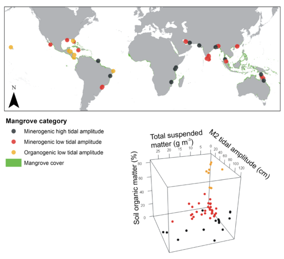
Key findings

Their results show that sites with SOM > 60% were found mostly in the Caribbean, Hawaii and Florida. Sites elsewhere had average OM values of ~10%, and thus broad description of mangrove soils as “peat” is misleading.

The broad majority of mangrove soils globally are minerogenic.

They then describe a variety of relevant mangrove restoration and management techniques relevant for the various mangrove geomorphic settings.

In organogenic settings, key risk is collapse of peat following disturbance. Influences on root productivity such as nutrient availability as well as inundation levels are of key importance.

They note that low tidal ranges often indicate the importance of seasonal flooding to the site. Management and restoration in microtidal sites is thus often concerned with preserving networks of terrestrial freshwater sources.

Minerogenic sites require high levels of sediment input to maintain intertidal surfaces at correct elevation relative to tidal frame, and thus proper management of hydroperiod at rates which mangroves prefer. Disturbances in sediment supply may influence long term health of mangroves. Use of bamboo fences in Vietnam and Thailand may help to reduce tidal energy and wave energy and promote sediment deposition.

Interesting that they note the Chao Phraya river has undergone a ~75% reduction in sediment yield, with severe coastal erosion resulting.

References

Hess, Laura L, John M Melack, and David S Simonett. 1990. “Radar Detection of Flooding Beneath the Forest Canopy: A Review.” International Journal of Remote Sensing 11 (7): 1313–25.

Walsh, Stephen J, David R Butler, and George P Malanson. 1998. “An Overview of Scale, Pattern, Process Relationships in Geomorphology: A Remote Sensing and Gis Perspective.” Geomorphology 21 (3-4): 183–205. doi:10.1016/S0169-555X(97)00057-3.

Imhoff, Marc Lee, and Dean B Gesch. 1990. “The Derivation of a Sub-Canopy Digital Terrain Model of a Flooded Forest Using Synthetic Aperture Radar.” Photogrammetric Engineering and Remote Sensing 56 (8): 1155–62.

Souza-Filho, Pedro Walfir Martins, and Waldir Renato Paradella. 2002. “Recognition of the main geobotanical features along the Bragança mangrove coast (Brazilian Amazon Region) from Landsat TM and RADARSAT-1 data.” Wetlands Ecology and Management 10: 123–32. doi:10.1023/a:1016527528919.

Souza-Filho, P W M, and W R Paradella. 2003. “Use of synthetic aperture radar for recognition of Coastal Geomorphological Features, land-use assessment and shoreline changes in Bragança coast, Para, Northern Brazil.” Anais Da Academia Brasileira De Ciencias 75 (3): 341–56. doi:10.1590/S0001-37652003000300007.

Knight, Jon M, Pat ER Dale, John Spencer, and Lachlan Griffin. 2009. “Exploring Lidar Data for Mapping the Micro-Topography and Tidal Hydro-Dynamics of Mangrove Systems: An Example from Southeast Queensland, Australia.” Estuarine, Coastal and Shelf Science 85 (4): 593–600. doi:10.1016/j.ecss.2009.10.002.

Smith, MJ, and CF Pain. 2009. “Applications of Remote Sensing in Geomorphology.” Progress in Physical Geography 33 (4): 568–82. doi:10.1177/0309133309346648.

Balke, Thorsten, and Daniel A Friess. 2016. “Geomorphic Knowledge for Mangrove Restoration: A Pan-Tropical Categorization.” Earth Surface Processes and Landforms 41 (2): 231–39. doi:10.1002/esp.3841.